Entscheidungsbäume mit CODAP
1. Entscheidungsbäume mit binären Daten
Basisfunktionen - Entscheidungsbäume mit arbor erstellen und interpretieren
In diesem Video wird gezeigt, wie mit Hilfe von CODAP ganz einfach datenbasierte Entscheidungsbäume per Drag & Drop erstellt werden können.
Mit folgendem Link gelangst du in die im Video genutzte CODAP Umgebung: https://tinyurl.com/CODAPEntscheidungsbaum

Mit dem Laden des Videos akzeptieren Sie die Datenschutzerklärung von YouTube.
Mehr erfahren
Maschine spielen - Entscheidungsbäume systematisch erstellen und dokumentieren
In diesem Video wird gezeigt, wie der in den vorherigen Items beschriebene Algorithmus in CODAP umgesetzt werden kann, sodass man gewissermaßen “Maschine spielt”.
Der Ansatz dabei ist, dass der Algorithmus durch Schülerinnen und Schüler semi-autmatisch durchgeführt wird, sodass sie die systematische Vorgehensweise handelnd verinnerlichen können.
Mit folgendem Link gelangst du in die im Video genutzte CODAP Umgebung: https://tinyurl.com/CODAPEntscheidungsbaum

Mit dem Laden des Videos akzeptieren Sie die Datenschutzerklärung von YouTube.
Mehr erfahren
Testen mit Testdaten - Entscheidungsbäume systematisch evaluieren
Lorem ipsum dolor sit amet, consectetur adipiscing elit. Ut elit tellus, luctus nec ullamcorper mattis, pulvinar dapibus leo.

Mit dem Laden des Videos akzeptieren Sie die Datenschutzerklärung von YouTube.
Mehr erfahren
Pruning - Entscheidungsbäume systematisch optimieren
Lorem ipsum dolor sit amet, consectetur adipiscing elit. Ut elit tellus, luctus nec ullamcorper mattis, pulvinar dapibus leo.

Mit dem Laden des Videos akzeptieren Sie die Datenschutzerklärung von YouTube.
Mehr erfahren
2. Entscheidungsbäume mit beliebigen Daten
Einen eigenen Datensatz in CODAP importieren
Das Arbor Plugin für Entscheidungsbäume importieren
Lorem ipsum dolor sit amet, consectetur adipiscing elit. Ut elit tellus, luctus nec ullamcorper mattis, pulvinar dapibus leo.

Mit dem Laden des Videos akzeptieren Sie die Datenschutzerklärung von YouTube.
Mehr erfahren
Ein CODAP Dokument per Link teilen
2.1 Elementarisation of machine learning with data-based DTs
ML, as described by Shalev-Shwartz & Ben-David (2014) and Hastie et al. (2009), is a heterogeneous field that includes different methods and learning algorithms for solving different types of tasks automatically in a statistical learning framework. The unifying element between all methods is that they are based on training data. We focus on the subspecies of supervised ML, specifically on classification tasks that can be addressed with DTs. The first contribution of this paper is the elementarised presentation of a data-based DT construction process that simplifies selected aspects of professional DT algorithms so that it is suitable for teaching in school and still serves as an example for ML. Our teaching unit and the research approach will be outlined later based on this elementarisation.
2.1.1 The statistical learning framework for creating classifiers
Classification involves the task of providing objects or individuals of a population with (ideally) correct labels concerning a certain question. In statistics, a population is a set of individuals, objects, or events that are of interest to a particular question or statistical investigation. (Kauermann & Küchenhoff, 2011, p. 5). Typical classification problems are assigning a patient with a diagnosis or classifying emails as “spam” or “not spam.” The possible labels come from a label set, depending on which we speak of a binary classification problem (two possible labels) or a multiclass classification problem (a finite set of more than two labels). The statistical learning framework is constituted by two main aspects that are described in the following (F1 and F2):
- F1 – Creating a classifier based on training data
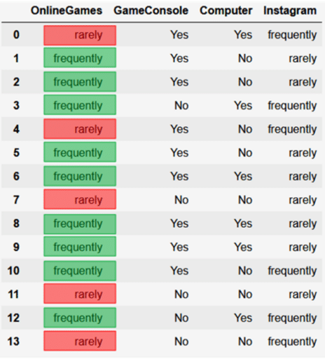
In a statistical learning framework, the task of a learning algorithm is to create a classifier that predicts a label for any given object in the population. The labels are values of a so-called target variable. To make an informed prediction, an object is represented by a set of characteristics displayed as a vector (called instance) from an input space. Since the characteristics inform the choice of the predicted label, they are called predictor variables. The creation of a classifier is based on training examples, i.e., objects from the population from which predictor variables’ values and correct labels are known. A set of training examples is called training data that can be represented in a data table, as illustrated below (Figure 2).
- F2 – Evaluating a classifier based on test data
As a measure of success in a statistical learning framework, the aim is to quantify the error of a classifier, which is the probability that it does not predict the correct label on a randomly chosen object from the population. Practically, the error is estimated by using test data to calculate the misclassification rate. Test data is structurally identical to training data but was not used to create the classifier.
2.1.2 Data-based construction of DTs as classifiers
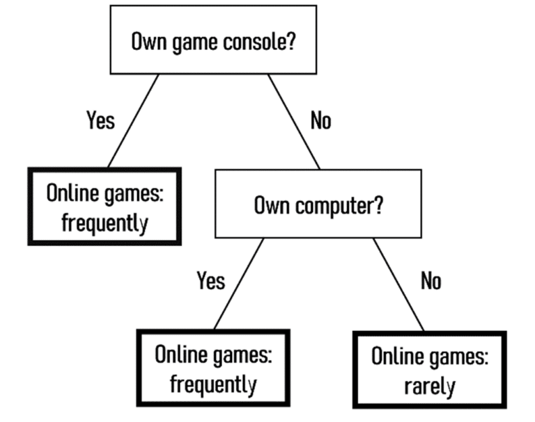
As characterized by Shalev-Shwartz & Ben-David (2014, p. 212), a DT is a type of classifier that predicts the label of an object by using a hierarchical structure of decision rules that progress from a root node of a tree to leaf nodes. At each node on the root-to-leaf path, the successor child node is chosen on the basis of a splitting of the input space. The internal nodes of the decision tree (excluding the leaf nodes) are referred to as split nodes. Each split node utilizes one of the predictor variables to divide the data. A leaf node always contains a label. This is exemplified by the simple DT in Figure 1 for the context of online platforms predicting whether users play online games frequently or rarely based on ownership of digital devices. The data-based creation of DTs is described below.

Figure 1: DT for predicting the frequency of online gaming
In the following, we consider the case of binary classification problems with binary predictor variables. Subsequent generalization to any form of categorical and numerical predictor variables is not difficult. We stay with the example of an online platform, which has a population of users about which some characteristics (types of digital devices used, frequency of platform use, etc.) are known. The platform recommends content to its users based on the topics they are interested in, one of which may be online gaming. Therefore, the task is to classify a user as “frequently” or “rarely” playing online games based on the characteristics known to the platform. For illustration, we use a mini sample of the JIM-PB data on adolescents’ media behaviour collected in the ProDaBi project (Podworny et al., 2022). The data sample in Figure 2 contains 14 cases and four binary variables.

Figure 2: JIM-PB Data sample 1
Characteristics include GameConsole and Computer ownership and the frequency of use of Instagram and OnlineGames, coded binary as frequently (at least once a week) or rarely.
Zero-level DT
The easiest possible DT would be just one node, which is both the root node and the leaf node, receiving the majority label of all 14 training examples. The frequency distribution in the training data in Figure 2 is “9 to 5”, i.e., for the target variable, there are nine occurrences of the value frequently and 5 of the value rarely. A “zero-level” DT simply provides every instance with the majority label (OnlineGames = frequently). The misclassification rate (MCR), referring to the training data, is calculated as the proportion of minority labels, which is 5 of 14 (35.7%) and can be used as a reference for the evaluation of one-level and multi-level DTs.
One-level DT
To create, evaluate, and represent a one-level DT based on training data, four process components (C1 – C4) can be distinguished.
- C1 – Performing a data split
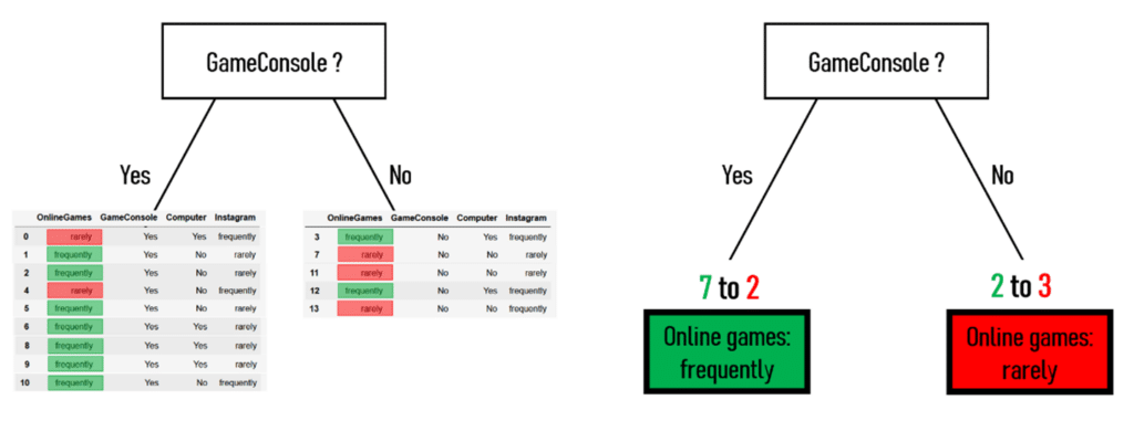
First, a so-called data split (C1) is done, producing two subsets of the training data by using a predictor variable and assigning every training example to a subset depending on the value of this predictor variable, as exemplified in Figure 3.
- C2 – Deriving a one-level DT from a data split
In the second step, based on the data split, for both subsets, a predicted label is specified to create a decision rule (C2) using the majority label for each subset. Each (new) instance is provided with the majority label of the subset to which the instance is assigned. In Figure 3, this would be “If GameConsole = Yes, then OnlineGames = frequently” and “If GameConsole = No, then OnlineGames = rarely”.
- C3 – Evaluating a DT
For evaluating a one-level DT (C3), the MCR referring to the training data is calculated, which is 4 of 14 (28.6%) in this example.
- C4 – Representing a DT
Then, the one-level DT can be represented (C4) in different forms, one of which is a DT diagram or the verbal form as the “if, then” rule specified above.

Figure 3: Example of a data split
What was exemplified in Figure 3 for the predictor variable GameConsole can be done similarly for the other two predictor variables, and the evaluation can be documented for each, as shown in Table 1.
Table 1: Evaluation of three different predictor variables used for a data split
predictor variable | number of misclassifications | misclassification rate (MCR) |
GameConsole | 4 | 28,6 % |
Computer | 5 | 35,7 % |
5 | 35,7 % |
Based on this documentation, we can conclude that using GameConsole yields the best-performing one-level DT for this training data with respect to MCR.
Die Seite befindet sich im Aufbau. Hier werden in Zukunft noch Inhalte ergänzt.
Hier geht es zu einer Unterrichtsreihe, die die gezeigten Inhalten behandelt: LINK


